Show the code
library(tidyverse)
library(haven)
library(ggplot2)
library(dplyr)
library(foreign)
library(readr)Is everyone getting taller? To find out, I combined five height studies published in five different formats: two Stata files, a zipped dBase (DBF) file, a CSV, and an SPSS survey. Each one used different column names, units, and age definitions. I standardized birth year and height (in inches and centimeters), kept only the comparable fields, and stacked the sources into a single tidy dataset.
library(tidyverse)
library(haven)
library(ggplot2)
library(dplyr)
library(foreign)
library(readr)one <- read_dta('https://byuistats.github.io/M335/data/heights/germanconscr.dta')
two <- read_dta('https://byuistats.github.io/M335/data/heights/germanprison.dta')
zip_path <- file.path(tempdir(), 'Heights_south-east.zip')
download.file('https://byuistats.github.io/M335/data/heights/Heights_south-east.zip', zip_path, mode = 'wb')
unzip(zip_path, exdir = tempdir())
three <- read.dbf(file.path(tempdir(), 'B6090.DBF'))
three <- as_tibble(three)
four <- read_csv('https://raw.githubusercontent.com/hadley/r4ds/main/data/heights.csv')
five <- read_sav('https://www.ssc.wisc.edu/nsfh/wave3/NSFH3%20Apr%202005%20release/main05022005.sav')cleanone <- one %>%
select(bdec, height) %>%
rename(Birth_Year = bdec, Height_cm = height) %>%
mutate(Source = "German Conscription Data" )
cleantwo <- two %>%
select(bdec, height) %>%
rename(Birth_Year = bdec, Height_cm = height) %>%
mutate(Source = "German Prison Data")
cleanthree <- three %>%
select(GEBJ, CMETER) %>%
rename(Birth_Year = GEBJ, Height_cm = CMETER) %>%
mutate(Source = "Southeast German Data")
cleanfour <- four %>%
filter(sex == "male") %>%
transmute(Birth_Year = 1950 - age, Height_cm = height * 2.54, Source = "Labor Statistics Data")
cleanfive <- five %>%
transmute(Birth_Year = 1900 + as.numeric(DOBY),
Height_feet = as.numeric(RT216F),
Height_inches = as.numeric(RT216I),
Source = "Wisconsin Data") %>%
filter(Height_feet >= 4,
Height_feet <= 7,
Height_inches >= 0,
Height_inches <= 11) %>%
mutate(Height_cm = ((Height_feet * 12) + Height_inches) * 2.54) %>%
select(Birth_Year, Height_cm, Source)all_heights <- bind_rows(cleanone, cleantwo, cleanthree, cleanfour, cleanfive) %>%
drop_na(Birth_Year, Height_cm, Source)
all_heights# A tibble: 27,851 × 3
Birth_Year Height_cm Source
<dbl> <dbl> <chr>
1 1850 170. German Conscription Data
2 1850 156. German Conscription Data
3 1850 172. German Conscription Data
4 1850 168. German Conscription Data
5 1850 167. German Conscription Data
6 1850 160. German Conscription Data
7 1850 161. German Conscription Data
8 1850 162. German Conscription Data
9 1850 162. German Conscription Data
10 1850 170. German Conscription Data
# ℹ 27,841 more rowsIn the cleaning of this data I decided to get rid of everything but things involving birth years and observed heights. So I kept all ages, birthday years and heights in any metric. I had to do some manipulating to get the proper formats for inches and centimeters and for birth years but then combining them was relatively easy. Once they were all cleaned up it didn’t take long to get all of it into one dataset.
ggplot(all_heights, aes(x = Birth_Year, y = Height_cm, color = Source)) +
  geom_point(size = 0.5, alpha = 0.6) +
  labs(title = "Male Height by Birth Year",
    color = "Study") +
  theme_bw()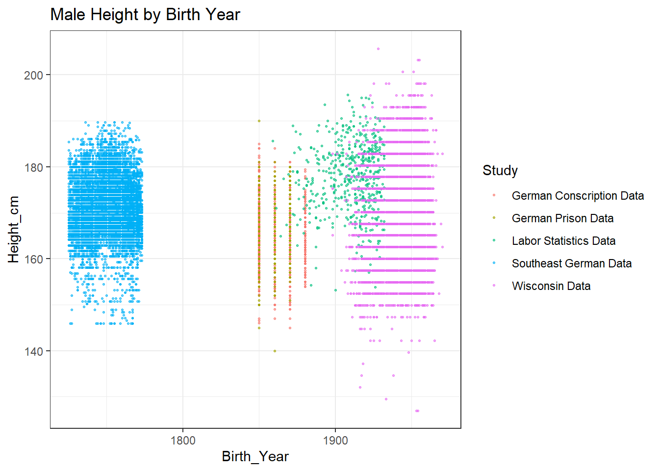
In the old data the trend was that people were getting taller over time. While data from the last activity backed this theory up, it was only one side of the story. We only had data at the time from one time period in one country. This let us see that people in Germany during the years 1810-1980 were in fact on average getting taller, but we can see a different trend in the data that we have availible now.
With this current data we can see many different peoples in different geographic locations and time periods mapped out over time. With this more cumulative dataset we can see that while people in Germany from 1810-1980 were in fact getting taller, the larger population of the world has not followed the same trend if you go back far enough. This is important because while it is interesting to follow trends and understand things within context windows, one cannot make a full generalization on everything based on such myopic data.