Car Wash Sales vs. Temperature

Overview

Does temperature drive car wash sales? I converted transaction timestamps from UTC to local time, removed invalid sales, and rolled them up to the hour. Then I pulled hourly weather observations for the Rexburg airport with the riem package and joined them to sales by hour.

library(tidyverse)
library(lubridate)
library(riem)
library(scales)

carwash_raw <- read_csv("https://byuistats.github.io/M335/data/carwash.csv")

carwash <- carwash_raw %>%
  mutate(UTC = ymd_hms(time, tz = "UTC"),
    local = with_tz(UTC, tzone = "America/Boise"))

ggplot(carwash, aes(x = amount)) +
  geom_histogram(bins = 30)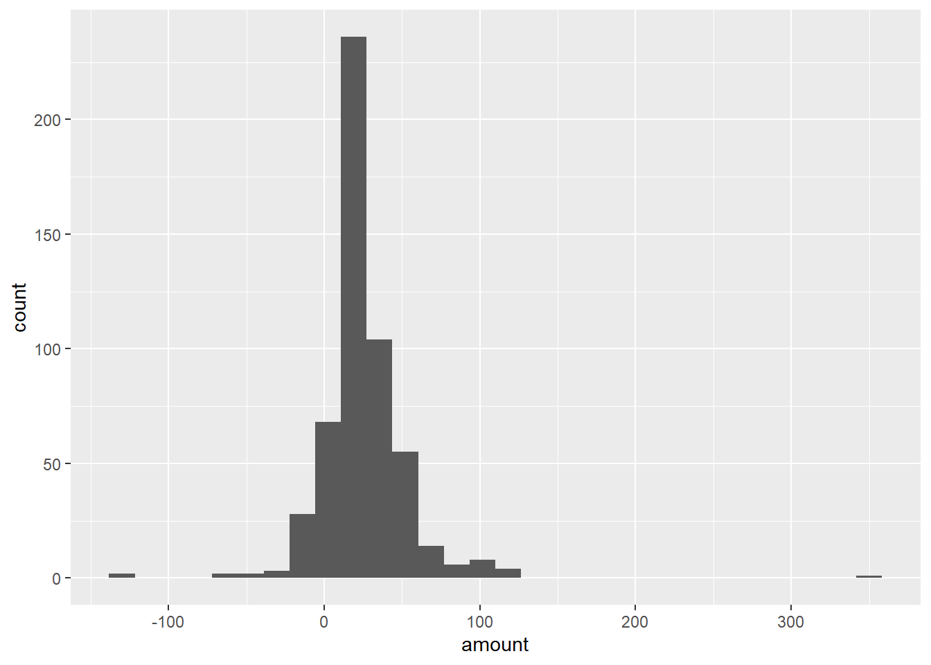

After inspecting the data, I decided to remove rows with missing time values, missing sale amounts, and negative sale amounts. I did not remove high sales just because they were high, because a large transaction could still be a real sale.

carwash_clean <- carwash %>%
  filter(
    !is.na(local),
    !is.na(amount),
    amount >= 0
  )

carwash_hourly <- carwash_clean %>%
  mutate(sales_hour = ceiling_date(local, unit = "hour"))

date_start <- min(as_date(carwash_hourly$sales_hour))
date_end <- max(as_date(carwash_hourly$sales_hour))

rexburg_weather_raw <- riem_measures(station = "RXE", date_start = date_start, date_end = date_end)

rexburg_weather_hourly <- rexburg_weather_raw %>%
  mutate(weather_time_local = with_tz(valid, tzone = "America/Boise"), 
         sales_hour = ceiling_date(weather_time_local, unit = "hour"))

carwash_weather <- carwash_hourly %>%
  left_join(rexburg_weather_hourly, by = "sales_hour")

carwash_weather_clean <- carwash_weather %>%
  filter(!is.na(tmpf))%>%
  mutate(hour_of_day = hour(sales_hour))

ggplot(carwash_weather_clean, aes(x = hour_of_day, y = amount, color = tmpf)) +
  geom_point(alpha = 0.65) +
  scale_y_continuous(labels = dollar_format()) +
  scale_x_continuous(breaks = seq(0, 23, by = 2)) +
  labs(
    title = "Car Wash Sales by Hour of Day",
    x = "Hour of day",
    y = "Total car wash sales per hour",
    color = "Temperature (F)"
  ) +
  theme_minimal()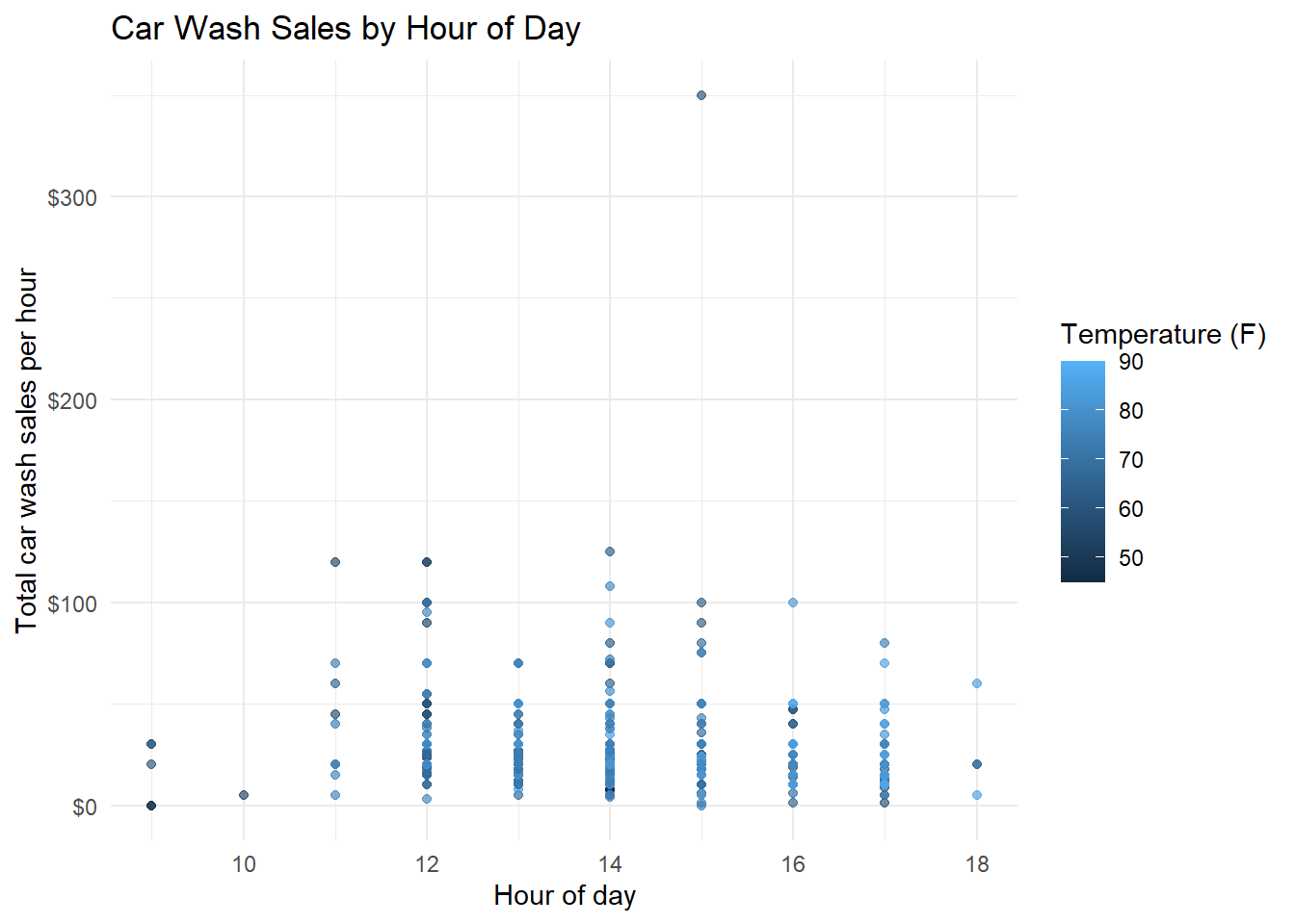

From the data we can see that the car wash has specific operating hours. This helps us to determine now when during those operating hours temperature and sales begin to influence one another. There seems to be no correlation of temperature and sales during operating hours. Sales peak in the morning, the middle of the day and the afternoon on different days. It would stand to reason though, from looking at the density of the data points on hotter days, that the warmer and more comfortable the day is, the more likely people are to go get a car wash.