Logistic regression modeling how the probability of scoring a water polo shot changes with distance from the goal.
R
Logistic Regression
Author
Spencer Payne
Background
In this analysis, the goal is to understand how the distance from the goal affects the likelihood that a water polo shot is successful or stated as a question, “Does distance affect whether a water polo player will make a shot in goal or not?” Each point represents a real shot attempt, recorded with a binary outcome. That the player scored (1) or did not score (0). Since the response variable is binary, a logistic regression model is appropriate. This approach allows us to estimate how the probability of scoring changes as the shooting distance increases. This model can show whether closer shots truly have a higher probability of success, and how sharply that probability declines as players shoot from farther away. Ultimately, the logistic model provides a way to quantify a common coaching belief in water polo: the farther the shot, the lower the chance it goes in.
Hypothesis
In our analysis, the probability that a shot is made based on the distance the player is from the goal is shown by this equation.
P(Y_i = 1|x_i) = \frac{e^{\beta_0+\beta_1 x_i}}{1+e^{\beta_0 + \beta_1 x_i}} = \pi_i
Using this model we can test if distance to the goal actually affects whether a shot is made or not. B_1 representing the effect that distance has on shooting percentage. We will be using an alpha of 0.05 to measure significance. Our null hypothesis stating that distance from the goal holds no effect on the probability of a successful shot. While our alternative hypothesis states that there is a relationship between the two.
H_0: \beta_1 = 0 \\
H_a: \beta_1 \neq 0\\
\alpha = 0.05
Analysis
Show the code
goal.glm <-glm(Binary_Goal ~as.numeric(DIST), data = wp, family = binomial)summary(goal.glm) %>%pander()
Estimate
Std. Error
z value
Pr(>|z|)
(Intercept)
0.7939
0.3627
2.189
0.02862
as.numeric(DIST)
-0.2981
0.08032
-3.711
0.0002066
(Dispersion parameter for binomial family taken to be 1 )
Null deviance:
285.8 on 214 degrees of freedom
Residual deviance:
270.8 on 213 degrees of freedom
P(Y_i = 1|x_i) \approx \frac{e^{0.7939-0.2981 x_i}}{1+e^{0.7939 - 0.2981 x_i}} = \hat{\pi}_i
This model and equation identifies that the intercept of the curve is at 0.7939 and that the slope is -0.2981. This means that we can tell that the farther the shooter moves from the goal the lower likelihood they have of making a successful shot. By a magnitude of 30% likelihood per meter away from the goal. The p-value for the slope is below the level of significance at 0.0002066 meaning that we can accept that the slope is different than 0 and therefore can reasonably accept the slope as we have it.
Graph
Show the code
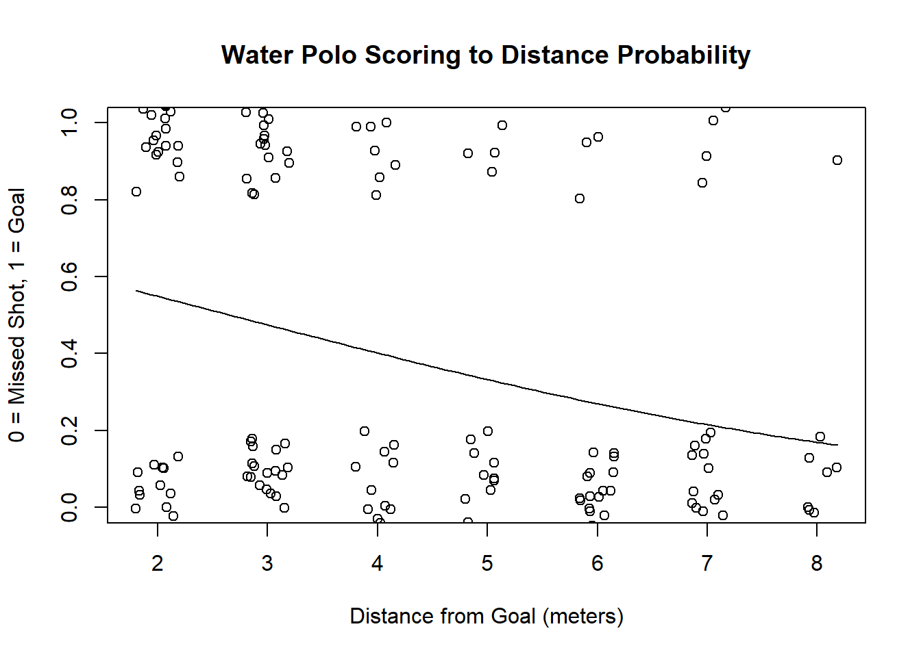
b <-coef(goal.glm)plot(jitter(Binary_Goal) ~jitter(DIST), data = wp, ylim =c(0,1), xlab ="Distance from Goal (meters)", ylab ="0 = Missed Shot, 1 = Goal", main ="Water Polo Scoring to Distance Probability")curve(exp(b[1] + b[2]*x) / (1+exp(b[1] + b[2]*x)), add =TRUE)
Show the code
pander(summary(goal.glm))
Estimate
Std. Error
z value
Pr(>|z|)
(Intercept)
0.7939
0.3627
2.189
0.02862
as.numeric(DIST)
-0.2981
0.08032
-3.711
0.0002066
(Dispersion parameter for binomial family taken to be 1 )
Null deviance:
285.8 on 214 degrees of freedom
Residual deviance:
270.8 on 213 degrees of freedom
By combining both the numerical summary and the graphic we can understand a little better the curve we have drawn for ourselves. The slop of -0.29 can be seen from the start and end of the curve which is validated by our p-value. Our intercept though is a little more difficult, the math shows us that it could be at 0.79. By interpreting the math into real world data we might say that if we were 0 meters away from the goal we would make it 80% into a successful goal which makes sense at least but it isn’t our main concern with the data.
Diagnosis
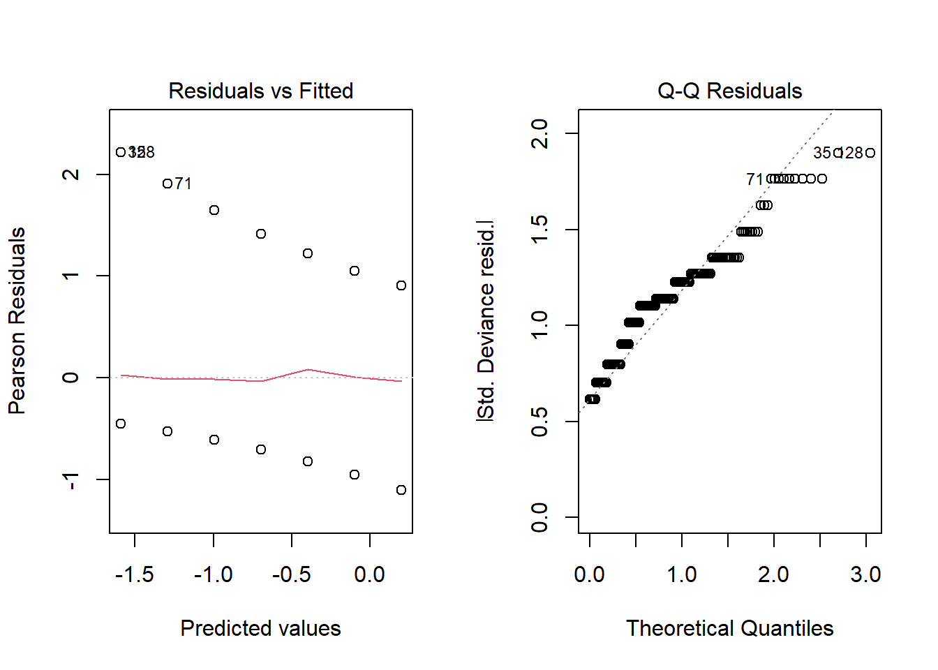
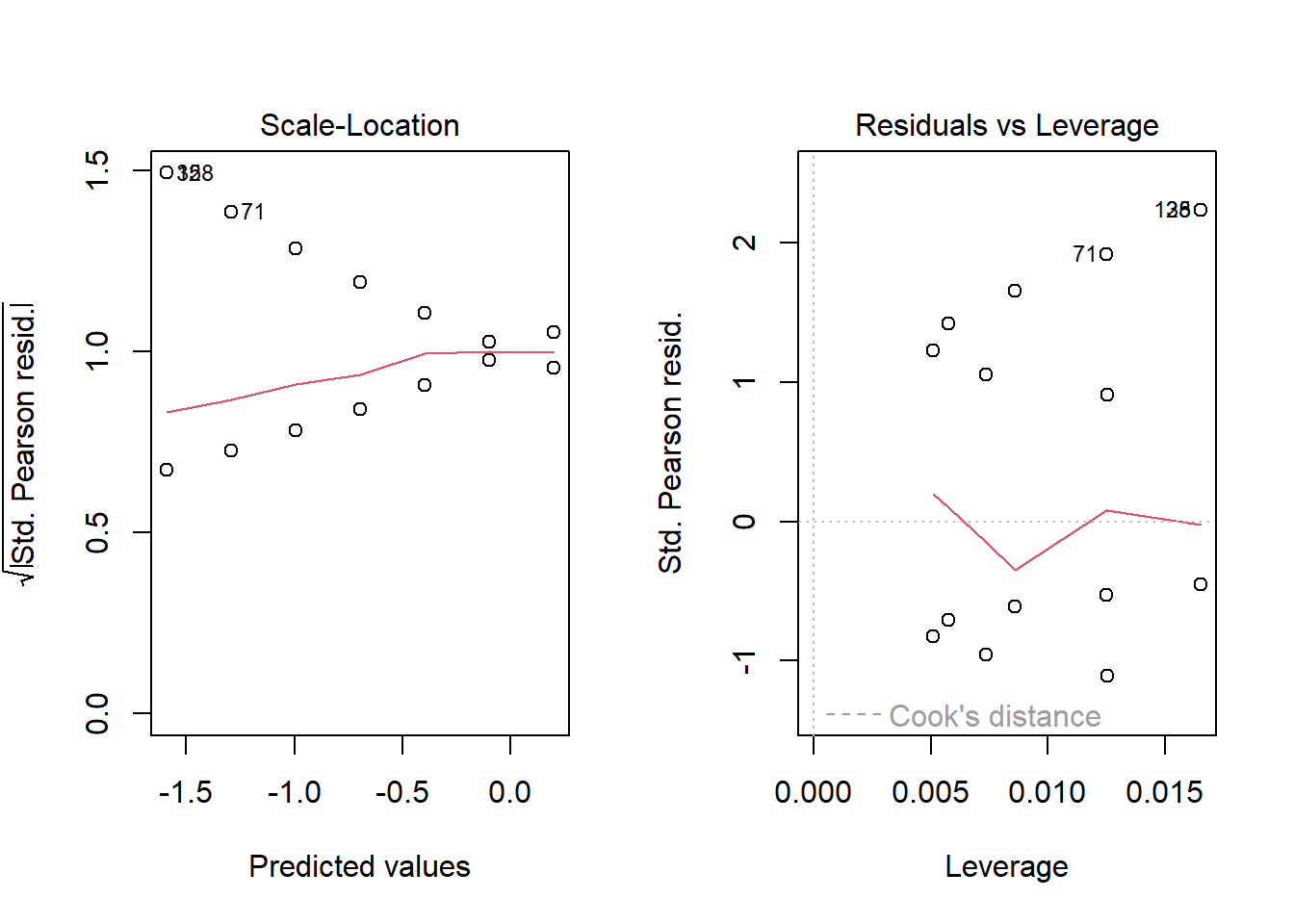
Doing a goodness of fit test on the data in the model we can see that it is very low at 0.004493372. This along with our various diagnostic graphs show us where our model left out important insights. For example, the QQ Plot shows us that the deviations in the data from what would be normally expected and the Residuals vs Fitted plot both under and over predicts the data. Overall, I don’t think it would be wise to treat the data as a huge source of truth within this analysis.
Show the code
par(mfrow=c(1,2))plot(goal.glm)
Show the code
pchisq(270.8, 213, lower.tail=FALSE)
[1] 0.004493372
Conclusion
Based on the logistic regression results, there is statistical evidence that distance from the goal has a meaningful effect on a player’s chance of scoring. The negative slope in the model indicates that as a shooter moves farther away from the goal, the probability of scoring steadily decreases. The p-value for the distance coefficient was well below the 0.05 significance level, allowing us to reject the null hypothesis and conclude that distance truly influences shot success. While the model does not perfectly predict outcomes, as shown by the low goodness-of-fit value, it still captures an important overall trend: close-range shots are much more likely to result in goals than long-range shots. In practical terms, this supports common coaching strategy in water polo, emphasizing high-percentage opportunities taken near the goal rather than low-percentage attempts from the perimeter. The analysis shows that distance matters, and the farther the shot, the slimmer the odds of scoring.