Caffeine, Distractions, and Reaction Time

Show the code

library(mosaic)
library(DT)
library(pander)
library(car)
library(tidyverse)
library(dplyr)
library(lattice)
library(lmtest)

# Record your data from your own mini experiment in Excel.
# Save the data as a .csv file in the Data folder of the Statistics-Notebook.

# Read in the data
Caff <- read_csv("data/MyTwoWayANOVA.csv")

Background and Hypothesis

The following data was taken from individuals to understand attention span and how things like external stimuli and caffeine can affect attention. The data was collected as subjects participated in tests designed to show subjects reaction time. Each participant took the test with and without caffeine and with and without external stimuli. Caffeine content ranged from 0mg, 50mg, and 100mg, each taken 45 min prior to engaging with the test. External stimuli consisted of no stimuli, audio stimuli (in the form of random pop songs), visual stimuli (in which subjects watched a video of ping pong practice), and combined audio and visual stimuli (where both the video and the music were played).

Show the code

knitr::kable(head(Caff))

Participant	Caffeine_mg	Distraction	Reaction_Time_ms
Alice	0	None	325
Alice	0	Audio	360
Alice	0	Visual	350
Alice	0	Audio+Visual	395
Alice	50	None	280
Alice	50	Audio	300

Show the code

Caff <- Caff %>%
  mutate(Distraction = factor(Distraction,
                              levels = c("None", "Audio", "Visual", "Audio+Visual"))) %>% 
  mutate(Caffeine_mg = factor(Caffeine_mg, 
                              levels = c("0", "50", "100")))

Of the whole experiment, two factors can effect the reaction time of the participants which are caffeine intake and stimuli. An ANOVA test will be performed on the data using the following hypothesis

H_0: \mu_\text{0mg} = \mu_\text{50mg}= \mu_\text{100mg}

H_a: \text{At least one } \mu \text{ differs among caffeine levels}

H_0: \mu_\text{None} = \mu_\text{Audio}= \mu_\text{Visual} = \mu_\text{Audio+Visual}

H_a: \text{At least one distraction mean differs}

(\alpha\beta)_\text{ij}= 0

(\alpha\beta)_\text{ij} \neq 0

\alpha = 0.05

Analysis

The analysis goes as follows

Show the code

Caff.aov <- aov(Reaction_Time_ms ~ Distraction + Caffeine_mg, data=Caff)
summary(Caff.aov)

            Df Sum Sq Mean Sq F value   Pr(>F)    
Distraction  3  25521    8507   42.08 1.02e-12 ***
Caffeine_mg  2  18154    9077   44.90 3.72e-11 ***
Residuals   42   8492     202                     
---
Signif. codes:  0 '***' 0.001 '**' 0.01 '*' 0.05 '.' 0.1 ' ' 1

By understanding the p-values we can see that each of the factors and their levels have a significant effect on the reaction time of the participants, each being below the level of significance. Distraction at 0.00000000000102 and caffeine at 0.0000000000372

Graphical Summaries

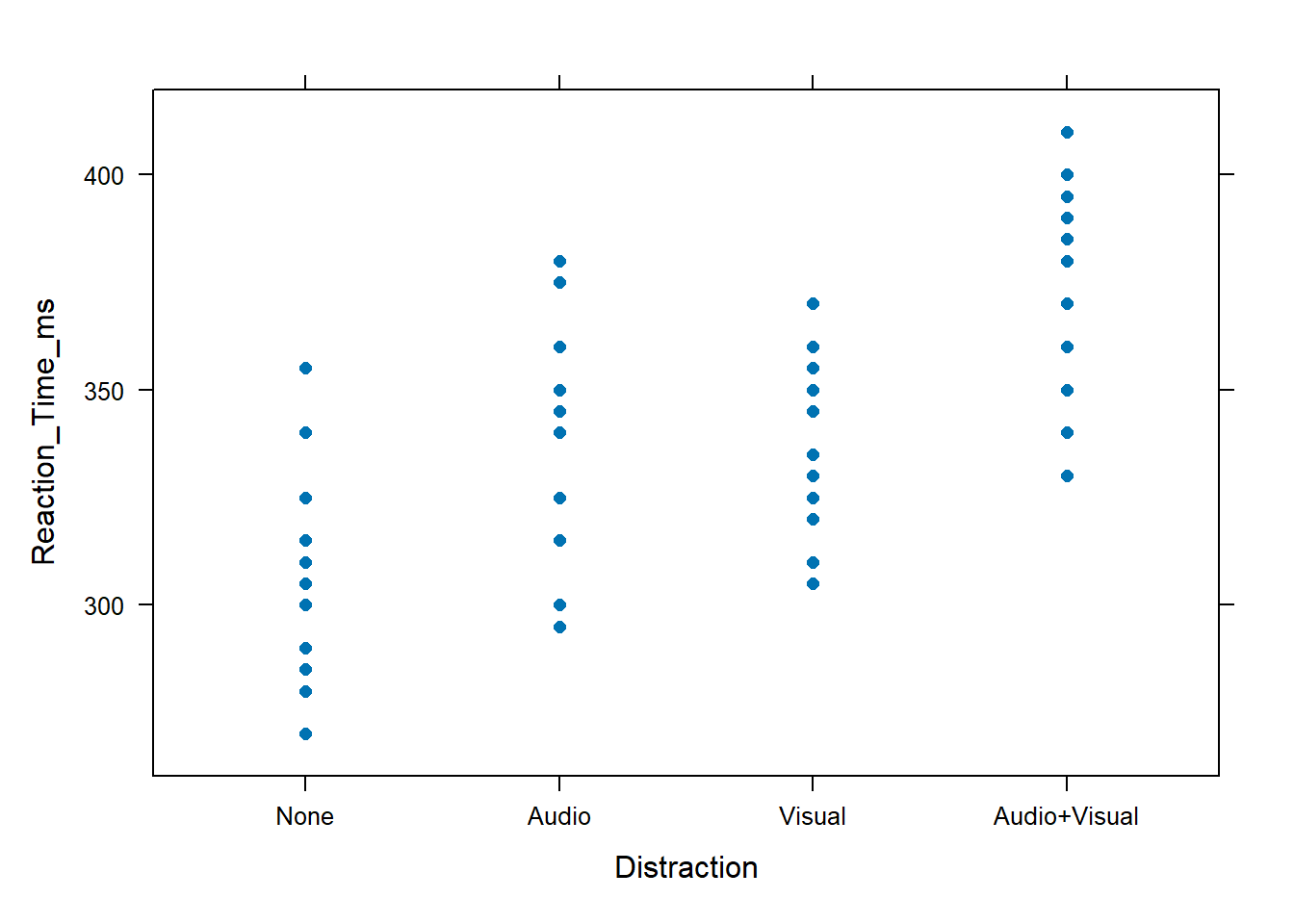
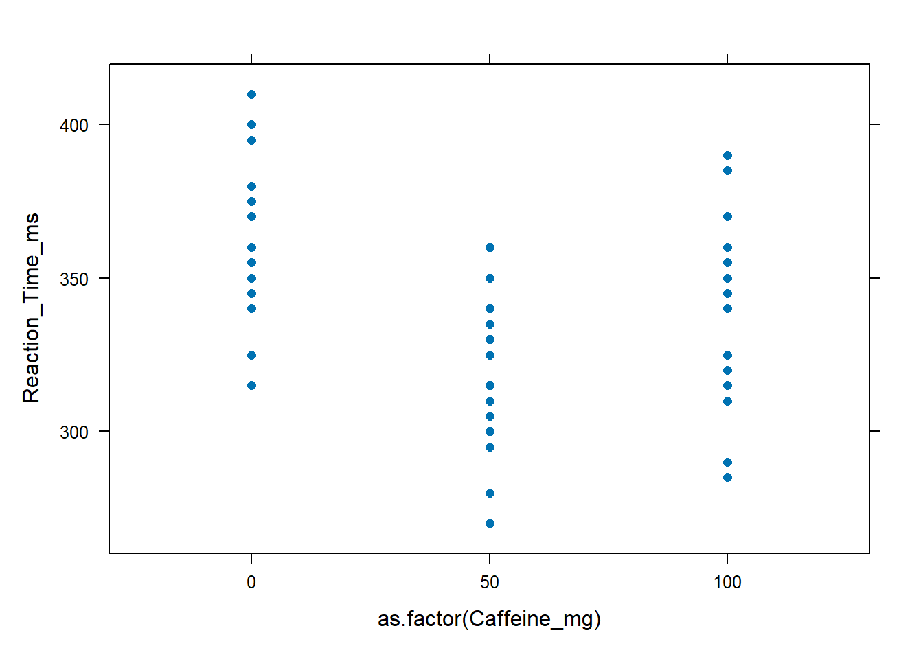
Modeling the results on using plots for each factor will aid in understanding the results of the ANOVA test.

Show the code

xyplot(Reaction_Time_ms ~ Distraction, data=Caff, main="", pch=16)

Show the code

xyplot(Reaction_Time_ms ~ as.factor(Caffeine_mg), data=Caff, main="", pch=16)

These graphs show us the effect that each of the factors and its levels have individually on the reaction times.

Diagnostic Plots

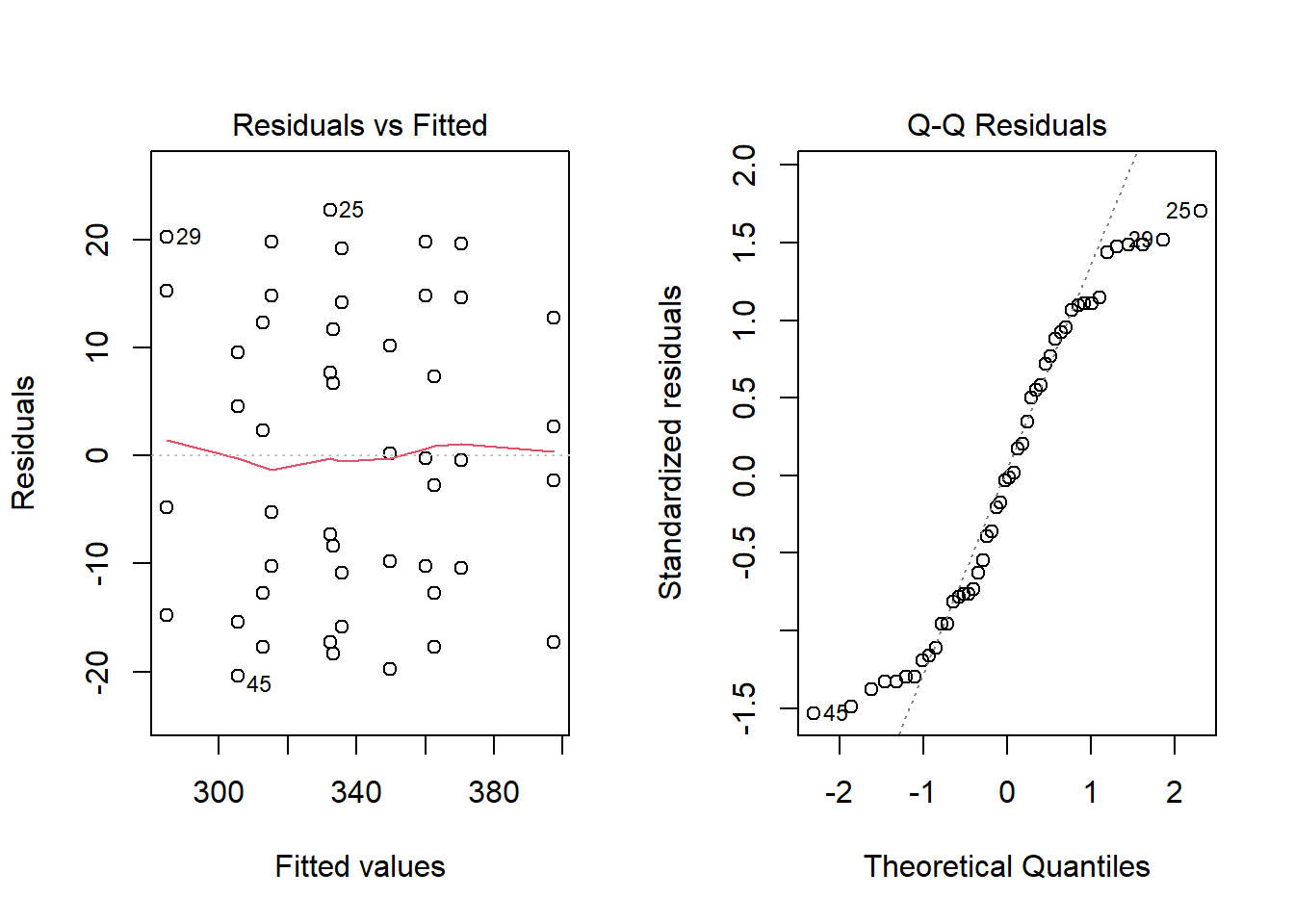
To check the normality of the data and assure ourselves that the ANOVA is valid we can check the residuals and QQPlot as is shown below.

Show the code

par(mfrow=c(1,2))
plot(Caff.aov, which=1:2)

Conclusion

Each of these summaries come together to show us the understanding we need about our data and the relationship each factor has with the others. Our diagnostic plots show us the data we have collected from our participants is usable and consistent with general population data. This helps us to understand the validity of the further analysis we have done on the data. Our XYPlots help to show us the rough relationship that distractions and caffeine levels have with reaction times. Hypothesizing from the graphic plots we can go forward in our analysis. After concluding that we believe that their is a relationship between reaction time and caffeine intake levels and reaction time and outside distraction, we move onto our analysis. say that, using a two-way ANOVA, caffeine and different distraction inputs have a significant relationship on reaction time.