Atmospheric Pressure and Temperature by City

Background

Readily available weather data can tell us a lot about the long term and short term weather conditions of a location based off of different attributes of the landscape. In this study we are going to be analyzing the relationship between atmospheric pressure and average temperature. Taking 3 different cities into account with varying elevations, climates and locations, we will attempt to understand how average temperature changes with air pressure. Our 3 locations in particular are Mexico City (CDMX), Rexburg, Idaho and Burbank, California. Mexico City has an elevation of 7349 feet. Rexburg has an elevation of 4862 feet. Burbank has an elevation of 600 feet.

Show the code

library(GSODR) #run: install.packages("GSODR") 
# to get the GSODR package. You'll need this package to pull in your weather data.
load(system.file("extdata", "isd_history.rda", package = "GSODR"))
library(dplyr)
library(pander)
library(stringr)
#Run this in your console to see the Country Names you can pick from:
#Search "United States" in the search bar of the top-right corner of the data Viewer that pops up.
#Or search for any other country you are interested in.
#Goal, select the STNID (station ID) for two different weather stations. 
#For example, Rexburg is STNID == "726818-94194"
#Once you have two STNID values selected, go to the next R-chunk.
rexburg <- get_GSOD(years = 2023, station = "726818-94194")
#Run: View(rexburg)
#To see what columns mean, go here: https://cran.r-project.org/web/packages/GSODR/vignettes/GSODR.html#appendices

burbank <- get_GSOD(years = 2023, station = "722880-23152")

CDMX <- get_GSOD(years = 2023, station = "766793-99999")

#Then run a similar code to get your station information for your weather stations.
#(If you want to use rexburg, then just use one of the following codes)
#cityName1 <- get_GSOD(years = 2023, station = "yourchoice1")
#cityName2 <- get_GSOD(years = 2023, station = "yourchoice2")

#Finally, join your two datasets together into one dataset:
raw <- rbind(rexburg, burbank, CDMX)
weather <- raw %>%
  mutate(
    name_clean = case_when(
      str_detect(NAME, regex("REXBURG", ignore_case = TRUE)) ~ "Rexburg",
      str_detect(NAME, regex("BURBANK", ignore_case = TRUE)) ~ "Burbank",
      str_detect(NAME, regex("BENITO", ignore_case = TRUE)) ~ "CDMX",
      TRUE ~ NAME   # fallback: keep original if none match
    )
  ) %>%
  # reorder so the new clean column comes first
  select(name_clean, everything(), -NAME)

In performing this analysis we must create an equation to map our data onto. This shape takes the form of a line that can be represented in the following equation.

Y_i = \beta_0 + \beta_1 X_{i1} + \beta_2 C_{i2} + \beta_3 C_{i3} + \beta_4(P_i * C_{i2}) + \beta_5(P_i * C_{i3}) + \epsilon_i Y_i represents the y value of the equation and the average temperature of the city.

Beta_0, Beta_2 and Beta_4 represent the various y intercepts for each city. Meaning that if the atmospheric pressure were 0, where might the average temperature lie. This idea helps us to test if our findings are true using the following hypothesis

H_o: \beta_0 = \beta_2 = \beta_4\\ H_a: \text {At least one } \beta_j \text { different}

Beta_1, Beta_3 and Beta_5 represent the slopes of each of the lines. If each city had a different rate of change to the relationship between average temperature and atmospheric pressure we would see it occur in these variables. This knowledge will help us with another hypothesis shown below.

H_o: \beta_1 = \beta_3 = \beta_5\\ H_a: \text {At least one } \beta_j \text { different}

We will also use an alpha of 0.05 so determine if a certain statistic is significant or not. \alpha = 0.05

Analysis

Show the code

weatherlm <- lm(formula = TEMP ~ SLP + name_clean + SLP:name_clean, data = weather)
pander(summary(weatherlm))

	Estimate	Std. Error	t value	Pr(>\|t\|)
(Intercept)	664.2	91.03	7.297	5.715e-13
SLP	-0.6379	0.08975	-7.108	2.14e-12
name_cleanCDMX	-2.732	129.9	-0.02103	0.9832
name_cleanRexburg	69.42	100.8	0.6884	0.4914
SLP:name_cleanCDMX	0.0008341	0.1284	0.006497	0.9948
SLP:name_cleanRexburg	-0.0758	0.09936	-0.7629	0.4457

Fitting linear model: TEMP ~ SLP + name_clean + SLP:name_clean
Observations	Residual Std. Error	R^2	Adjusted R^2
1081	6.264	0.4977	0.4954

Show the code

b <- coef(weatherlm)

We can see from the above analysis that we can safetly assume that the original line for our Burbank data is correct with a y intercept of 664.2 and a slope of -0.64 and a p value way below the level of significance. The other lines though have levels of significance way above what we can tolerate. While their information is valueable and puts us on a good track for further study, it would be unwise to trust the results. This may have been because the other two cities have elevations way above Burbank and other factors like winds and other geographic landmarks may interrupt the average temperature.

Graph

Show the code

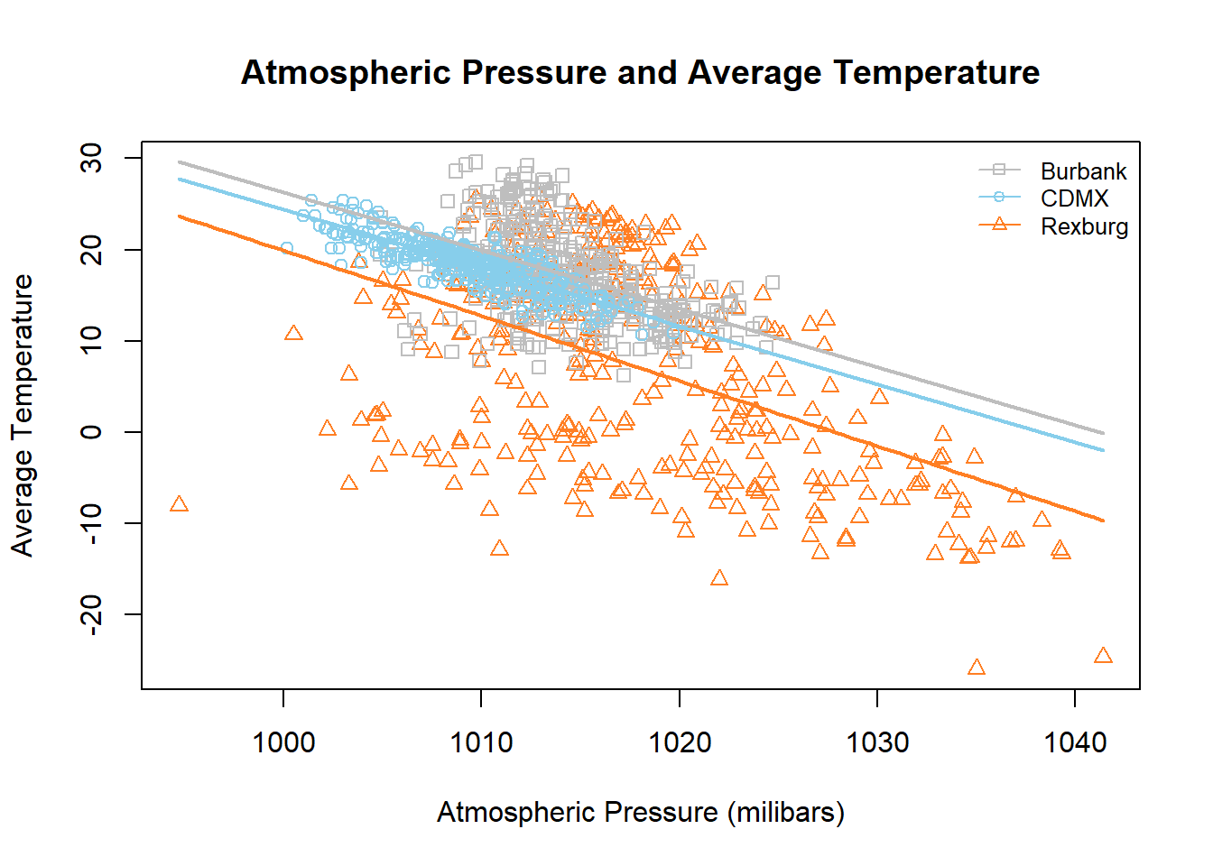
palette(c("grey", "skyblue", "chocolate1"))
plot(TEMP ~ SLP, data = weather, col = as.factor(name_clean), pch = c(0,1,2)[as.factor(name_clean)], main = "Atmospheric Pressure and Average Temperature", xlab = "Atmospheric Pressure (milibars)", ylab = "Average Temperature" )
legend("topright", legend = c("Burbank", "CDMX", "Rexburg"), bty = "n", lty = 1, col = palette(), cex = 0.8, pch = c(0, 1, 2))
curve(b[1] + b[2]*x, col = palette()[1], lwd = 2, add = TRUE)
curve((b[1] + b[3]) + (b[2] + b[5])*x, col = palette()[2], lwd = 2, add = TRUE)
curve((b[1] + b[4]) + (b[2] + b[6])*x, col = palette()[3], lwd = 2, add = TRUE)

The above graph shows us the reality of the data we have collected. Understanding the analysis helps us to narrow down useful data without putting too much stock into the data point for the other cities. The grey points and line are aspects that have a reasonable level of significance for the data. Which, now that we are looking at the data points makes sense because the points for Rexburg are so spread out and the one for CDMX is so clustered together. Only Burbank has data points sufficient to create a cohesive line.

Diagnosis

Show the code

par(mfrow = c(2, 2))
plot(weatherlm)

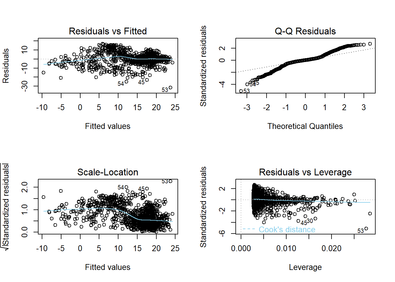
The diagnostic plots, at an overview, show us a little of what we have seen in the analysis which is that a lot of the data doesn’t support the results that we have. For example, the QQ Plot follows the diagnostic line at some points but most of it falls way outside the range that might be considered reliable data. The same could be said for the Scale-Location and Residual vs. Fitted graphs.

Conclusion

Our original research question was whether atmospheric pressure and average temperature had a significant relationship within 3 different cities. Our results showed us the significant relationship they had at a city with lower altitude but could not find a relationship between the two at higher altitudes. We can safety say that in Burbank, CA, atmospheric pressure and average temperature have a negative linear relationship. For further study it might be pertinent to filter out all data but from Burbank, CA so that we might know with a higher certainty the relationship between the two without the data from the other cities to influence the diagnostic plots as we have seen in this analysis.