Show the code
library(tidyverse)
library(sf)
library(USAboundaries)
library(geofacet)
library(scales)
library(viridis)
library(buildings)

data("permits")How hard did the 2008 housing crisis hit new construction? Using U.S. Census building permit data, I calculated the percent change in single-family permits from 2006 to 2010. I mapped it by state with sf and then zoomed into California counties, using a diverging color scale so that declines and increases stand out.
library(tidyverse)
library(sf)
library(USAboundaries)
library(geofacet)
library(scales)
library(viridis)
library(buildings)
data("permits")state_permits <- permits %>%
filter(variable == "Single Family")california_county_permits <- permits %>%
filter(variable == "Single Family") %>%
filter(StateAbbr == "CA")us_states <- us_states() %>%
filter(stusps != "PR" & stusps != "HI" & stusps != "AK")
ca_counties <- us_counties(states = "California")state_permits <- state_permits %>%
mutate(state_fips = str_pad(state, width = 2, pad = "0"))
california_county_permits <- california_county_permits %>%
mutate(state_fips = str_pad(state, width = 2, pad = "0")) %>%
mutate(county_fips = str_pad(county, width = 3, pad = "0")) %>%
mutate(full_county_fips = paste0(state_fips, county_fips))state_permits_map <- us_states %>%
mutate(state_fips = statefp) %>%
left_join(state_permits, by = "state_fips")
ca_county_permits_map <- ca_counties %>%
mutate(full_county_fips = geoid) %>%
left_join(california_county_permits, by = "full_county_fips")state_change <- state_permits %>%
group_by(state_fips, StateAbbr, year) %>%
summarize(total_permits = sum(value, na.rm = TRUE), .groups = "drop") %>%
filter(year %in% c(2006, 2010)) %>%
pivot_wider(names_from = year, values_from = total_permits,
names_prefix = "permits_") %>%
mutate(percent_change = (permits_2010 - permits_2006) / permits_2006)state_change_map <- us_states %>%
mutate(state_fips = statefp) %>%
left_join(state_change, by = "state_fips")ggplot(state_change_map) +
geom_sf(aes(fill = percent_change), color = "white", linewidth = 0.2) +
scale_fill_gradient2(low = "red", mid = "white", high = "blue", midpoint = 0,
labels = percent_format()) +
labs(title = "Single Family Building Permits Nationwide",
subtitle = "% change from '06 to '10",
fill = "% change") +
theme_classic()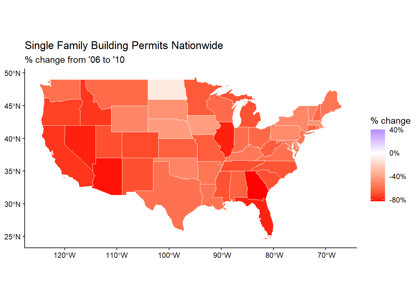
ca_county_change <- california_county_permits %>%
  group_by(full_county_fips, year) %>%
  summarize(total_permits = sum(value, na.rm = TRUE), .groups = "drop") %>%
  filter(year %in% c(2006, 2010)) %>%
  pivot_wider(names_from = year, values_from = total_permits,
    names_prefix = "permits_") %>%
mutate(percent_change = (permits_2010 - permits_2006) / permits_2006)ca_county_change_map <- ca_counties %>%
mutate(full_county_fips = geoid) %>%
left_join(ca_county_change, by = "full_county_fips")ggplot(ca_county_change_map) +
geom_sf(aes(fill = percent_change), color = "white", linewidth = 0.2) +
scale_fill_gradient2(low = "red", mid = "white", high = "blue", midpoint = 0,
labels = percent_format()) +
labs(title = "Single Family Building Permits by County in CA",
subtitle = "% change from '06 to '10",
fill = "% change") +
theme_classic()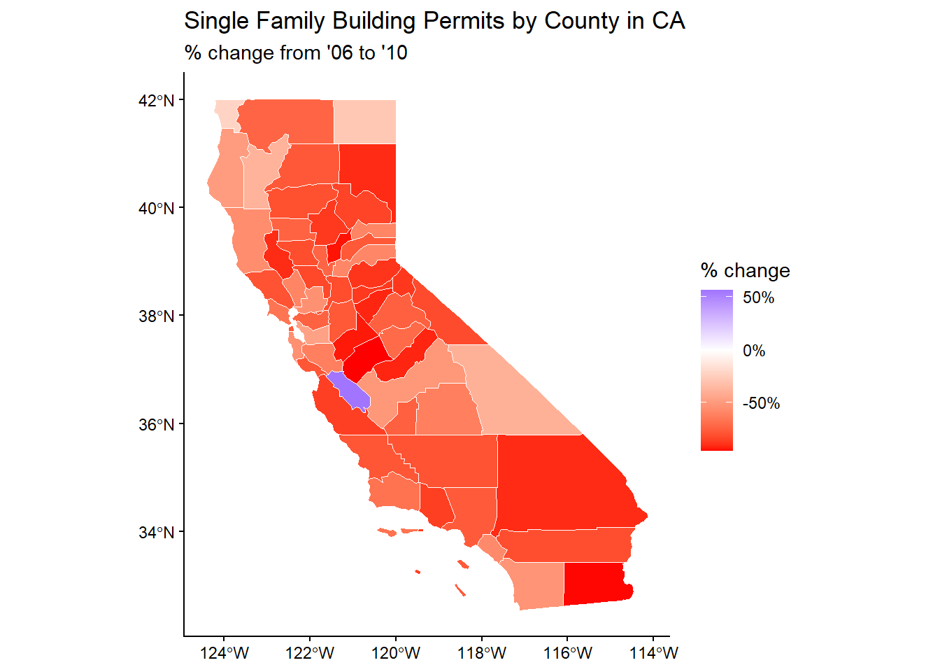
These graphics show the trend of single family building permits in the US and California specifically from 2006-2010 following and after the mortgage crisis. In each graph we can observe that the largest majority of geographical areas at both the state and national level fell by a large margin, with only very specific and select places not falling too much or increasing in one particular area.
In organizing this data I chose to focus on California because it is my home state and because it has San Jose, California which is a huge place for Silicon Valley which seemed to do alright despite the crisis. In filtering the data I only included the continental united states. I also wanted to emphasize the the negative and positive trends over everything else so that’s why no change is a neutral white.